Normal Approximation to Binomial Distribution

Example Binomial Distribution

A Binomial Distribution is great for finding probabilities of "Yes/No" events (like coin flips).

But what if we flip that coin 100 times? The calcs gets hard. Fast.

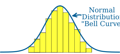
Luckily, big binomial graphs start looking like a smooth bell. We can use the Normal Distribution instead. It gives us a close answer, way faster:

When Can We Use It?

We shouldn't use this approximation if the data is too skewed (lopsided).

A good rule of thumb is that we can use it when both:

• np ≥ 5
• n(1 − p) ≥ 5

(Where n is the total number of trials and p is the probability of success)

Setting the Parameters

To use the Normal curve, we need to find the Mean (μ) and Standard Deviation (σ) from our Binomial data:

The Continuity Correction

The Binomial distribution is discrete (it has separate bars for 0, 1, 2, and so on.), but the Normal distribution is continuous (a smooth line).

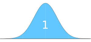
Normal Distribution
Area = 1
Certain to be in there

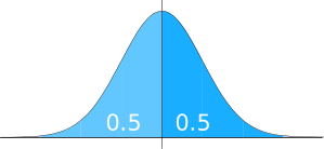
Normal Distribution
Area = 0.5 + 0.5 = 1
50% chance of each side

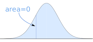
Area at a value is zero
Probability of exactly that value

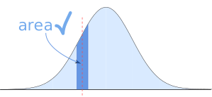
Area belonging to value
Probability of being "in the bin"

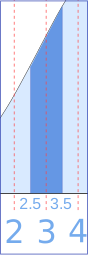
Example:

A Binomial value of 3 becomes a Normal Distribution area between 2.5 and 3.5

We use 0.5 because the Binomial steps go by 1. The bin stretches halfway to its neighbors. Let's try a full example.

Example: Flipping a Coin

We flip a fair coin 100 times. What's the probability of getting exactly 45 heads?

• Check:
  • n=100
  • p=0.5
  • np=50
  • n(1−p)=50
  both np and n(1−p) are greater than 5, so we are good to go.
• Find μ and σ:
  • μ = 100 × 0.5 = 50
  • σ = √(100 × 0.5 × 0.5) = 5
• Apply Correction: For "Exactly 45", we look for the area between 44.5 and 45.5
• Get Z-scores:
  • Z₁ = (44.5 − 50) / 5 = −1.1
  • Z₂ = (45.5 − 50) / 5 = −0.9
• Look up Area:
  • Find the area between Z = −1.1 and Z = −0.9 using the Standard Normal Distribution table
  • 1.1 →0.3643, and 0.9 →0.3159
  • the area in between is 0.3643 − 0.3159 = 0.0484, which is 4.84%

What about Ranges?

When we want a range of values, like "More than 3" or "At least 3", we just have to decide which bin edges to use:

• More than 3: We want 4, 5, 6... so we start at 3.5
• At least 3: We want 3, 4, 5... so we start at 2.5 (including 3's bin)
• Less than 3: We want 0, 1, 2... so we end at 2.5
• At most 3: We want 0, 1, 2, 3... so we end at 3.5 (including 3's bin)

Don't Memorize the Rules

Instead of memorizing which way to add or subtract 0.5, draw a quick sketch!

Draw a number line, draw a little box around your target numbers (extending 0.5 on each side)

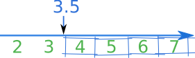
More than 3

Now you can see right away where the range starts and/or stops.

Summary

• When n is large, the Binomial Distribution looks similar to the Normal Distribution
• This makes the math way easier, and the answer is very close